Intro to Raster Analytics
The Raster Analytics service is a powerful imagery processing API designed for users to build and run analytics that work at any scale. Raster Analytics provides direct, scalable, high-performance access to imagery for any area-of-interest (AOI) with dynamic on-the-fly processing. The processing capabilities of the Raster Analytics service are provided by the Image Processing Engine (IPE). IPE includes all the undifferentiated geospatial heavy lifting imagery preprocessing, corrections, and enhancements needed to make the raster data suitable for both on-screen visualization and automated analysis. By using the Raster Analytics service you get access to the exact imagery data and analytics results you need when you need it with minimal setup required.
The Raster Analytics service cuts out the need to order, download, and manage any images as files. With the service you can simply discover the images you wish and then directly access the images via the service.
The Raster Analytics service introduces the idea of a virtual GeoTIFF file. This virtual GeoTIFF works exactly like a GeoTIFF file stored on a disk, but it is "virtualized" by the service in an on-demand basis. Like all GeoTIFF images, the virtual GeoTIFF has header information and all the other content of a GeoTIFF Image. It is intended that the end-users will access our virtual GeoTIFF via standard clients like GDAL, OpenLayers, and GeoTIFF.js. These clients can make calls to our Raster Analytics service using range reads and will present our virtual GeoTIFF images in standard ways like any other GeoTIFF image on disk.
Getting Started Tutorial: Accessing Images with GDAL
Required installs:
Set your api key
maxar_api_key="<YOUR API KEY>"
This API key will be used in all requests to the Raster Analytics API as a query string parameter. To provision an API key, please reference the Authentication documentation.
Searching the Catalog for available images
To access an image with the Raster Analytics API it must be available in the catalog in the cloud-optimized-archive collection. You can use the Discovery API to search for available images or confirm that an image is available.
Search the cloud-optimized-archive Collection with filters for a list of available catalog identifiers
curl --request POST "https://api.maxar.com/discovery/v1/search?maxar_api_key=$maxar_api_key" \
--header "Content-Type: application/x-www-form-urlencoded" \
--data "collections=cloud-optimized-archive" \
--data 'datetime=2025-03-25T00:00:00Z/..' \
--data "where=eo:cloud_cover < 10" \
--data "bbox=-105,40,-104,41" \
| jq '.features[] | .id'
"B140001100A49800"
"10300101116BC300"
"B13000110084E000"
"B13000110083D600"
"1030010110D69000"
"B13000110083AE00"
Check if an image is available in the cloud-optimized-archive Collection
collect_identifier="1040010083D45E00"
curl --request GET "https://api.maxar.com/discovery/v1/search?collections=cloud-optimized-archive&ids=$collect_identifier&maxar_api_key=$maxar_api_key" \
| jq 'if (.features[] | length) > 0 then .features[].id + " found" else empty end'
"104005004CDCAE00 found"
Getting the list of available bands from the catalog record
You will need to use the Discovery API to check an image's available bands for use with the Raster Analytics API.
curl --request GET "https://api.maxar.com/discovery/v1/search?collection=cloud-optimized-archive&ids=$collect_identifier&maxar_api_key=$maxar_api_key" \
| jq '.features[0] | .properties | .["eo:bands"][].name'
"red"
"red_edge"
"green"
"blue"
"yellow"
"nir2"
"nir1"
"pan"
"coastal"
For additional catalog query examples, reference the Discovery API docs
Monitoring for Raster Analytic Data Events
You can setup an monitor to notify you when data that fits your criteria is added to the Raster Analytics archive. See monitoring for details.
Raster Analytics API: Building a URL to a virtual GeoTIFF
Context
The Raster Analytics API presents available images as a virtual GeoTIFF. The images are virtual because they are created just-in-time, with output representation determined by a processing graph. The processing graphs are also dynamically instantiated per service request by reference to an Image Processing Engine Script (IPEScript). With IPEScript defined graphs being hugely customizable and the just-in-time nature of the processing, the Raster Analytics API can support a multitude of output representations for a given collect.
Working with IPEScript functions and their parameters
This tutorial will use an IPEScript named ortho that supports two functions to return orthorectified images. The below example demonstrates the optionality provided via these functions and their parameters. The complete ortho reference can be found here.
script_id="ortho"
Functions:
ortho: returns an orthorectified panchromatic or multispectral image
pansharp_ortho: returns an orthorectified pansharpened image
Each function has its own parameters. For example, pansharp_ortho supports the following:
function="pansharp_ortho"

# Required function parameters
collect_identifier="1040010083D45E00"
crs="UTM"

# Optional function parameters
bands="red,green,blue"
dra="true"
acomp="false"
hd="false"
The complete pansharp_ortho function parameter descriptions can be referenced here
Building a Raster Analytics API URL to a virtual GeoTIFF
We can now use the above script, selected function, and parameters to build a Raster Analytics API URL to a virtual GeoTIFF.
url="https://api.maxar.com/analytics/v1/raster/$script_id/geotiff?function=$function&p=collect_identifier=\"$collect_identifier\"&p=crs=\"$crs\"&p=bands=\"$bands\"&p=dra=$dra&p=acomp=$acomp&p=hd=$hd&maxar_api_key=$maxar_api_key"
echo $url
https://api.maxar.com/analytics/v1/raster/ortho/geotiff?function=pansharp_ortho&p=collect_identifier="1040010083D45E00"&p=crs="UTM"&p=bands="red,green,blue"&p=dra=true&p=acomp=false&p=hd=false&maxar_api_key=<YOUR API KEY>
Since you are going to use GDAL to access this virtual GeoTIFF you need to prepend the correct GDAL Virtual File System prefix to the URL. For the Raster Analytics API it will always be /vsicurl/.
gdal_url="/vsicurl/$url"
echo $gdal_url
/vsicurl/https://api.maxar.com/analytics/v1/raster/ortho/geotiff?function=pansharp_ortho&p=collect_identifier="1040010083D45E00"&p=crs="UTM"&p=bands="red,green,blue"&p=dra=true&p=acomp=false&p=hd=false&maxar_api_key=<YOUR API KEY>
For more information on building virtual GeoTIFF urls see our documentation here.
Accessing a virtual GeoTIFF with GDAL
Prior to using gdal_translate we can ensure the virtual GeoTIFF is valid and can be read in by GDAL with the gdalinfo program.
GDAL_DISABLE_READDIR_ON_OPEN=YES gdalinfo "$gdal_url"
Driver: GTiff/GeoTIFF
Files: /vsicurl/https://api.maxar.com/analytics/v1/raster/ortho/geotiff?function=pansharp_ortho&p=collect_identifier="1040010083D45E00"&p=crs="UTM"&p=bands="red,green,blue"&p=dra=true&p=acomp=false&p=hd=false&maxar_api_key=...
Size is 43762, 137641
Coordinate System is:
PROJCRS["WGS 84 / UTM zone 47N",
    BASEGEOGCRS["WGS 84",
        ENSEMBLE["World Geodetic System 1984 ensemble",
            MEMBER["World Geodetic System 1984 (Transit)"],
            MEMBER["World Geodetic System 1984 (G730)"],
            MEMBER["World Geodetic System 1984 (G873)"],
            MEMBER["World Geodetic System 1984 (G1150)"],
            MEMBER["World Geodetic System 1984 (G1674)"],
            MEMBER["World Geodetic System 1984 (G1762)"],
            MEMBER["World Geodetic System 1984 (G2139)"],
            MEMBER["World Geodetic System 1984 (G2296)"],
            ELLIPSOID["WGS 84",6378137,298.257223563,
                LENGTHUNIT["metre",1]],
            ENSEMBLEACCURACY[2.0]],
        PRIMEM["Greenwich",0,
            ANGLEUNIT["degree",0.0174532925199433]],
        ID["EPSG",4326]],
    CONVERSION["UTM zone 47N",
        METHOD["Transverse Mercator",
            ID["EPSG",9807]],
        PARAMETER["Latitude of natural origin",0,
            ANGLEUNIT["degree",0.0174532925199433],
            ID["EPSG",8801]],
        PARAMETER["Longitude of natural origin",99,
            ANGLEUNIT["degree",0.0174532925199433],
            ID["EPSG",8802]],
        PARAMETER["Scale factor at natural origin",0.9996,
            SCALEUNIT["unity",1],
            ID["EPSG",8805]],
        PARAMETER["False easting",500000,
            LENGTHUNIT["metre",1],
            ID["EPSG",8806]],
        PARAMETER["False northing",0,
            LENGTHUNIT["metre",1],
            ID["EPSG",8807]]],
    CS[Cartesian,2],
        AXIS["(E)",east,
            ORDER[1],
            LENGTHUNIT["metre",1]],
        AXIS["(N)",north,
            ORDER[2],
            LENGTHUNIT["metre",1]],
    USAGE[
        SCOPE["Navigation and medium accuracy spatial referencing."],
        AREA["Between 96°E and 102°E, northern hemisphere between equator and 84°N, onshore and offshore. China. Indonesia. Laos. Malaysia - West Malaysia. Mongolia. Myanmar (Burma). Russian Federation. Thailand."],
        BBOX[0,96,84,102]],
    ID["EPSG",32647]]
Data axis to CRS axis mapping: 1,2
Origin = (693351.330947023350745,1705842.718378915218636)
Pixel Size = (0.365366161666667,-0.365366161666667)
Metadata:
TIFFTAG_SOFTWARE=Transform-API modified Apache Commons Imaging
TIFFTAG_COPYRIGHT=Maxar Inc. 2025
VEHICLE_NAME=WV03
ACQUISITION_TIME=2023-03-30T03:47:31.437047Z
COLLECT_IDENTIFIER=1040010083D45E00
AREA_OR_POINT=Area
Image Structure Metadata:
INTERLEAVE=PIXEL
Corner Coordinates:
Upper Left  (  693351.331, 1705842.718) (100d48' 6.55"E, 15d25'20.24"N)
Lower Left  (  693351.331, 1655553.355) (100d47'52.68"E, 14d58' 4.25"N)
Upper Right (  709340.485, 1705842.718) (100d57' 2.74"E, 15d25'15.71"N)
Lower Right (  709340.485, 1655553.355) (100d56'47.72"E, 14d57'59.85"N)
Center      (  701345.908, 1680698.036) (100d52'27.37"E, 15d11'40.07"N)
Band 1 Block=256x256 Type=Byte, ColorInterp=Red
Description = red
Band 2 Block=256x256 Type=Byte, ColorInterp=Green
Description = green
Band 3 Block=256x256 Type=Byte, ColorInterp=Blue
Description = blue
Now that you have confirmed that GDAL recognizes the virtual GeoTIFF you have configured, it's time to access actual image data. A simple way to do that is to use the gdal_translate program.
First you should configure some useful GDAL environment variables.
export VSI_CACHE=TRUE
export VSI_CACHE_SIZE=500000000
export GDAL_HTTP_CONNECTTIMEOUT=60
export GDAL_NUM_THREADS=16
export GDAL_HTTP_TIMEOUT=60
export GDAL_HTTP_VERSION=2
export GDAL_HTTP_MULTIPLEX=YES
export GDAL_HTTP_MAX_RETRY=3
export GDAL_HTTP_RETRY_DELAY=5
export GDAL_HTTP_MULTIRANGE=YES
export GDAL_HTTP_MERGE_CONSECUTIVE_RANGES=NO
export GDAL_DISABLE_READDIR_ON_OPEN=YES
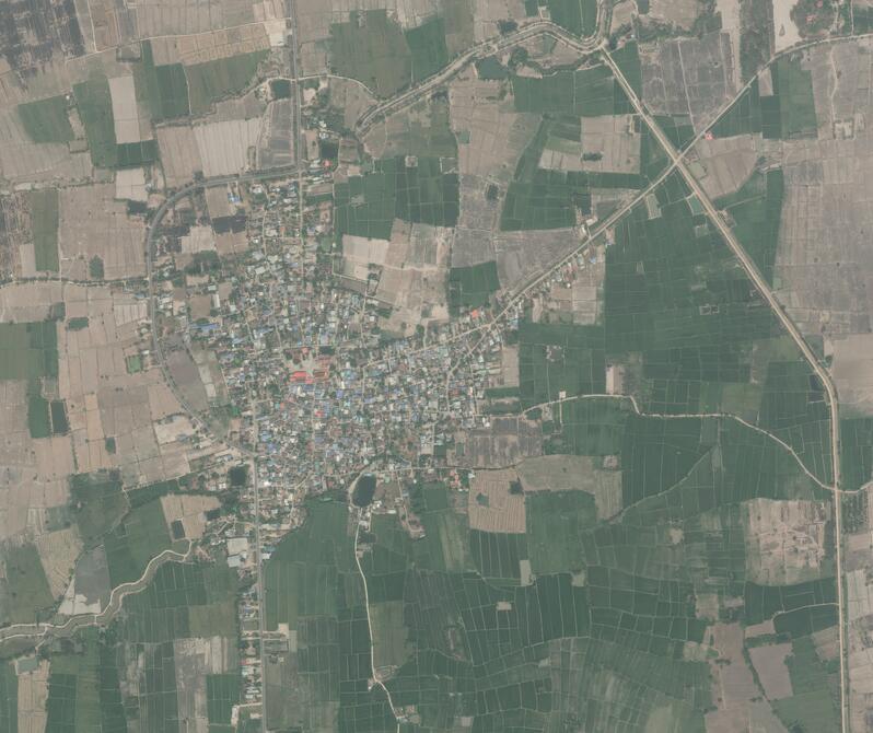
Extract an 8bit RGBN subwindow of the virtual GeoTIFF to current directory
projwin="100.831752 15.279735 100.854685 15.260719"
projwin_srs="EPSG:4326"
time gdal_translate $gdal_url "$(pwd)/${collect_identifier}_rgb_8bit.tif" -projwin $projwin -projwin_srs $projwin_srs
Input file size is 43762, 137641
0...10...20...30...40...50...60...70...80...90...100 - done.

real	3m7.648s
user	0m3.562s
sys	    0m0.997s
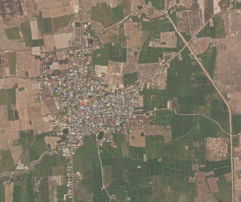
Produce the same image with atmospheric compensation
acomp="true"

gdal_url="/vsicurl/https://api.maxar.com/analytics/v1/raster/$script_id/geotiff?function=$function&p=collect_identifier=\"$collect_identifier\"&p=crs=\"$crs\"&p=bands=\"$bands\"&p=dra=$dra&p=acomp=$acomp&p=hd=$hd&maxar_api_key=$maxar_api_key"
time gdal_translate $gdal_url "$(pwd)/${collect_identifier}_rgb_acomp_8bit.tif" -projwin $projwin -projwin_srs $projwin_srs
Input file size is 43762, 137641
0...10...20...30...40...50...60...70...80...90...100 - done.

real	6m28.896s
user	0m3.768s
sys	    0m1.120s
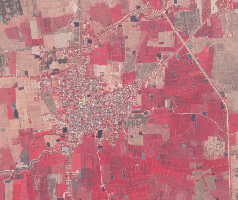
Extract an 8bit false color subwindow of the collect
bands="nir1,red,green"

gdal_url="/vsicurl/https://api.maxar.com/analytics/v1/raster/$script_id/geotiff?function=$function&p=collect_identifier=\"$collect_identifier\"&p=crs=\"$crs\"&p=bands=\"$bands\"&p=dra=$dra&maxar_api_key=$maxar_api_key"
time gdal_translate $gdal_url "$(pwd)/${collect_identifier}_nrg_acomp_8bit.tif" -projwin $projwin -projwin_srs $projwin_srs
Input file size is 43762, 137641
0...10...20...30...40...50...60...70...80...90...100 - done.

real	2m19.395s
user	0m3.516s
sys	    0m0.939s
Fetch all bands and full radiometric resolution in a 16bit subwindow of the collect
bands="coastal,blue,yellow,green,red,red_edge,nir1,nir2"
dra="false"

gdal_url="/vsicurl/https://api.maxar.com/analytics/v1/raster/$script_id/geotiff?function=$function&p=collect_identifier=\"$collect_identifier\"&p=crs=\"$crs\"&p=bands=\"$bands\"&p=dra=$dra&maxar_api_key=$maxar_api_key"
time gdal_translate $gdal_url "$(pwd)/${collect_identifier}_8_bands_16bit.tif" -projwin $projwin -projwin_srs $projwin_srs
Input file size is 43696, 134503
0...10...20...30...40...50...60...70...80...90...100 - done.

real	1m46.611s
user	0m12.435s
sys	    0m3.592s